Final Report

Project Summary

This project’s objective is to use machine learning algorithms to explore the supervised task of adding and removing rain from Minecraft scenes. Our initial objective was to build a model that converts a rainy Minecraft landscape image into a clear Minecraft image of the same landscape without rain. On the way, we also attempted to add rain effects to clear sky images. We also extended the model from still images to videos, by using consecutive frames of a video as input for the model.

This project will allow users to share gameplay in different environment conditions and showcase the effectiveness of machine learning algorithms in detecting and converting weather effects in a simulated realistic environment of Minecraft. With additional time and resources, this project could be applied to other sets of images, such as screenshots of other games or real life images. Being able to remove the visual effects of weather could be useful for people wanting to share images of scenery in situations where they cannot change the weather.

Approach

Our first task was to generate a collection of paired images depicting a given scene in two different conditions, rainy and clear weather. Using Malmo, we created a mission for the agent that uses chat commands to teleport him to random coordinates in the Minecraft World. Our script then takes a screenshot of the Minecraft client window, capturing what the agent sees, first with rainy weather. The code then uses another chat command to change the weather to clear weather; another screenshot is taken from the same position, capturing what the agent sees, under clear weather. Our collected images were manually sorted to remove useless images such as all black underwater images. We also have data of snow and desert areas with no rain, as these regions do not have those properties. All our current data is taken at noon in Minecraft time.

We collected and built our dataset by randomly teleporting the Malmo agent to random coordinates in a Minecraft world and taking screenshots with rainy and clear weather. Our dataset consists of 950 paired images, after filtering out underwater images and areas without rain.

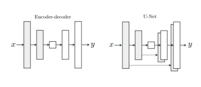
For our model, we took inspiration from an image to image translation GANs model. Since the combination of Malmo and Minecraft allowed us to generate paired data, we decided to use only the Generator to create a deep neural network with a U-Net architecture. This encoder and decoder structure of the U-net works to downsample and upsample the image with skip connections between mirrored layers as shown below from Phillip Isola’s paper. The layers are comprised of convolutions, rectifiers, and batch normalization. The encoder down samples the image to 1x1 through 8 blocks down and up samples back to 256x256 with 8 blocks up, gradually reducing the filter size as recommended in the referenced image to image translation paper.

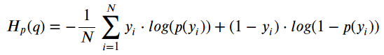
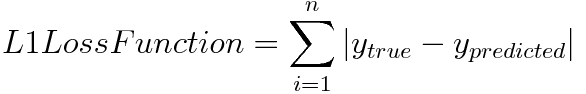
Once the layers are constructed, other parameters are set including the optimizer using Adam with a learning rate of 0.0001 and beta values of 0.5 and 0.999. The L1 loss function multiplied by a weight of 100 concatenated to the binary cross entropy loss is used (both equations listed below). Both loss functions are used because the BCE loss helps to smooth the images as it has a bias towards 0.5 while the L1 loss is used to maintain the original rgb of the input image.

Minecraft Video Footage

To see how our project could possibly be extended to video, we tried to remove rain weather effects from a video of Minecraft footage. Our input was a 90 second, 60 fps video of Minecraft gameplay, walking around the world in rainy weather. The video was broken into individual frames, which were then inputted into the model. Converted frames were then stitched back together to form a 90 second, 12 fps video of the same footage under clear weather conditions.

Some frames of the output video have white spots in the center or unremoved rain effects. This is likely because those frames were too different from the training data. Our training data looked straight ahead at the horizon over landscape; many frames of the test video looked up at the sky, directly at water (meaning the entire frame was blue) or was otherwise positioned in a way that the sun should not have been in the center. If we had more time and resources to build a larger and more diverse training dataset, it could have been possible to get better results here.

Evaluation

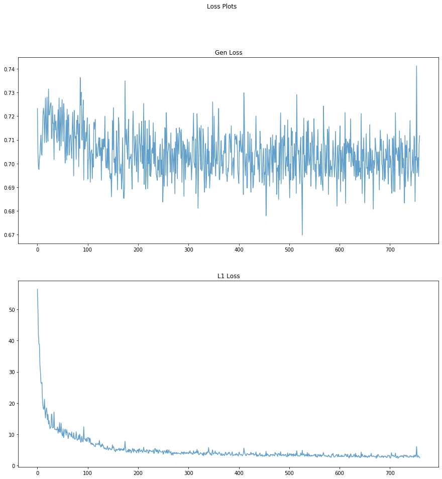
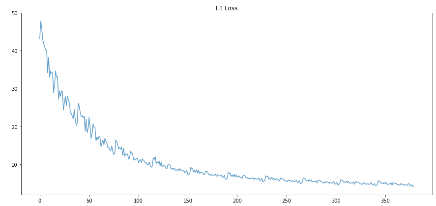
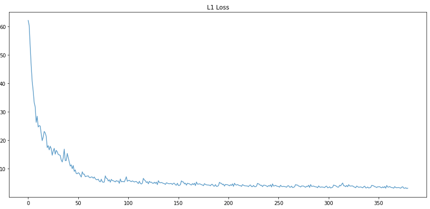
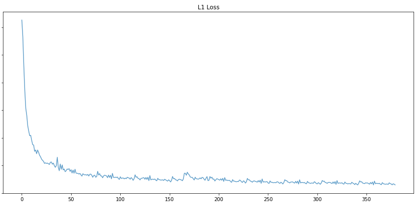
As a first step for evaluating our images, we checked the loss functions to make sure that they are decreasing. The binary cross entropy loss was not going down as much but we were able to see a drop in the L1 loss.

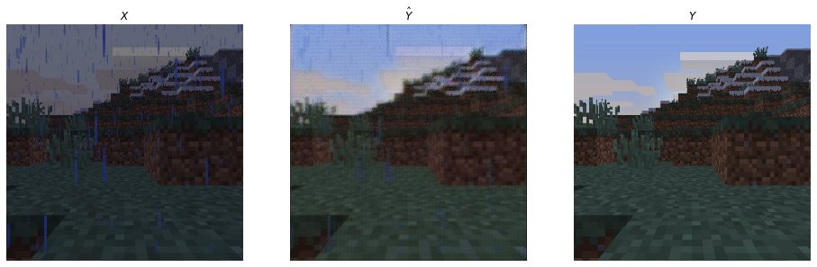
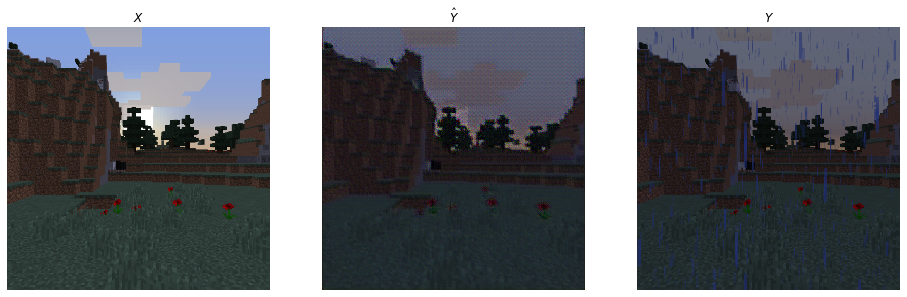
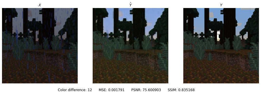
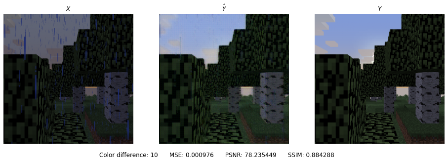
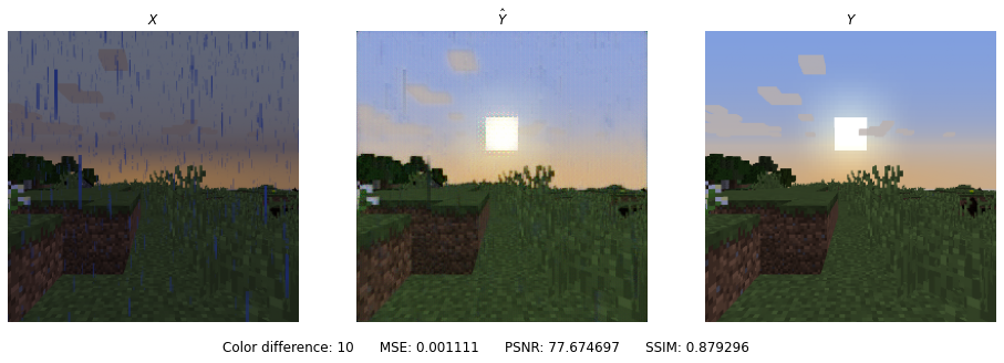
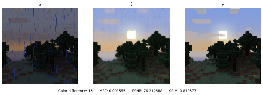
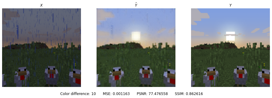
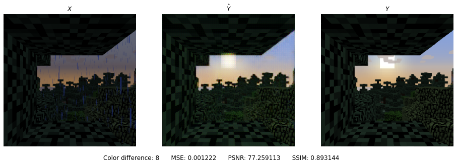
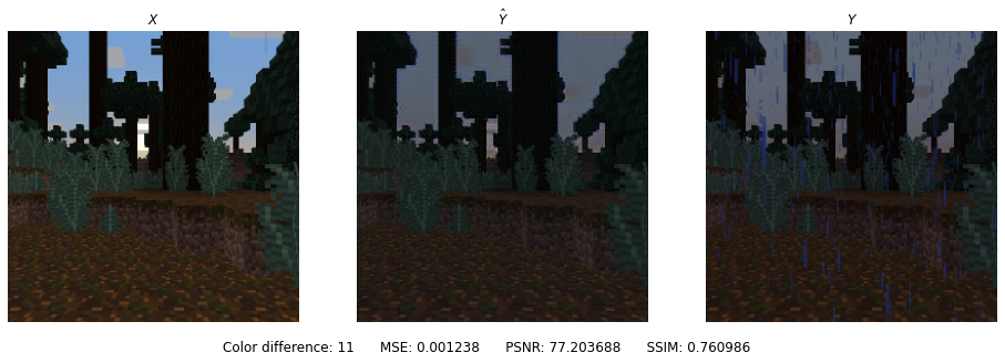
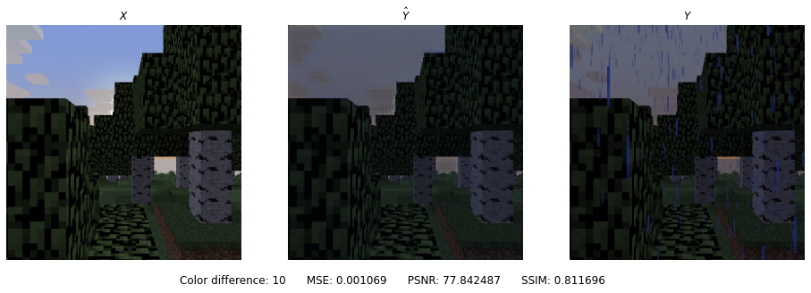
The second form of evaluation was through visually comparing side by side photos of the input, predicted, and target data. As seen below, the Minecraft rain images to sunny performed fairly well in removing the blue streaks. The images were slightly blurred because of the smoothing that occurs to remove the rain. The sunny to rain conversion was slightly more difficult for the model through visual inspection as the images were darkened for the rain effect but was not able to portray blue streaks.

Generated images for removing rain:

Inverse mapping of our model to add rain:

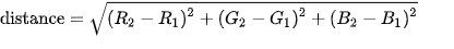
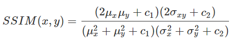
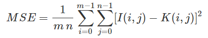
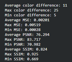
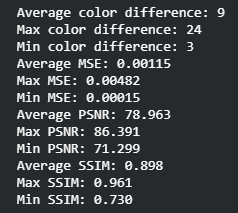
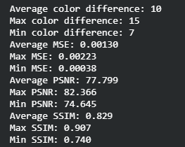
Originally, for qualitative measurements we were hoping to achieve a 50% pixel accuracy rate for the RGB channels but realized that this would not work considering that our model will predict float values in the 0~1 range that would be mapped to 0~255. For this reason, we have come up with alternative evaluation metrics: Color Distance, Peak Signal to Noise Ratio (PSNR), Structural Similarity Method (SSIM), and Mean Squared Error (MSE). Color distance is a variant of the Euclidean distance that measures the RGB distance for each pixel. PSNR and SSIM are metrics often used in image comparison. PSNR is based on MSE and is a ratio between the maximum amount of power and the distorted noise of an image. SSIM measures the perceptual difference based on luminescence, contrast, and structure. For Color Distance and MSE, the lower values perform better but for PSNR and SSIM, the higher values perform better.

Results from Experimentation

For the following experimentation, we kept all hyperparameters except one constant to see the effects of the changed hyperparameter.

Loss Functions

The loss function is derived from the Pixel to Pixel GANS model which multiples a lambda value of 100 to the L1 loss and concatenates it to BCE. Since this makes the L1 loss value extremely large, we believe that BCE has an insignificant effect on the loss function which is why it is unable to decrease as seen above. The BCE loss function was also run on its own but was not learning patterns, most likely because the L1 loss function maintains the original RGB of the input image. For this reason, we removed BCE and decided to only use the L1 loss.

Learning Rate

To find the ideal learning rate, we employed a similar strategy. We started with learning rate 1 and decreased by powers of 10. Learning rates 1 and 0.1 performed very poorly while learning rates 0.01, 0.001, and 0.0001 were able to learn the general shape of the image. We decided that learning rate 1e-3 or 0.001 is the best because the PSNR/SSIM are the highest (higher the better) and the color distance/MSE is the lowest in the sample prediction. The average values of the color difference, MSE, PSNR, and SSIM for all predictions were also very close for the later 3 so we decided on the middle learning rate.

Learning Rate	Sample Prediction	L1 Loss Function
1
0.1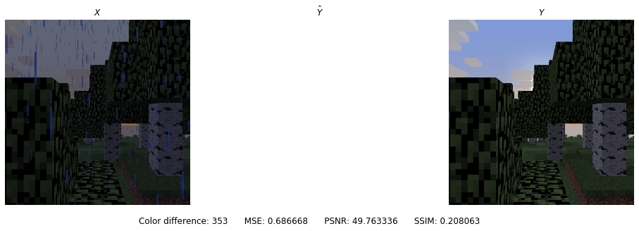
0.01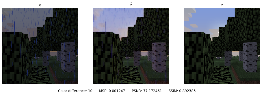
0.001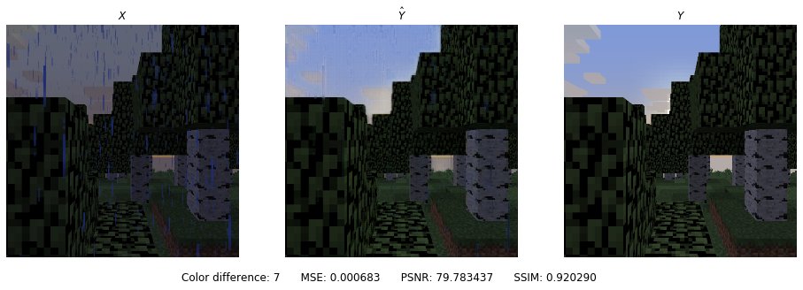
0.0001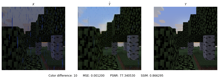

Batch Size

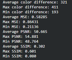
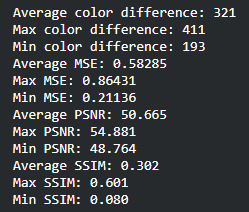
One of the hyperparameters of our model is batch size. To find the batch size that produced the best results, we tried training the model on batch sizes 5, 10, 20, and 40 and looked at the means of color distance, as well as MSE, PSNR, and SSIM of their test results. We found that batch size 5 was able to minimize color distance and MSE while maximizing PSNR and SSIM; we decided to use that value. Although batch size 5 was performing the best, batch size 40 performed the second best which shows that the model could have performed well on larger batch sizes. We would have run larger batch sizes if we could, but we were not able to due because our computers did not have enough GPU memory.

Batch Size	Sample Prediction	Data
5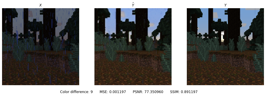
10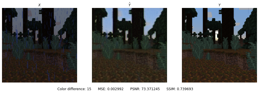
20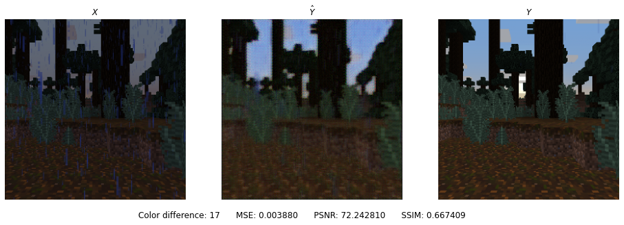
40

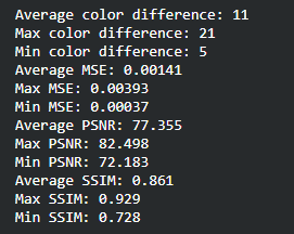
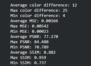
Filters

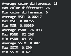
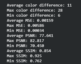
One of our most important experiments was with the model architecture itself: changing the number of filters in the last convolutional layer. This will make the model more complex, potentially allowing it to learn more patterns. We experimented with 16, 64, and 128 and found that the more complex the model got, the better predictions it was outputting. Just visually looking at the images, we can see the sharpness in the edges increase from 16 to 64 to 128. The evaluation metrics also showed improvement as color distance/MSE went down and PSNR/SSIM went up. This was a clear indication of improvement and we decided that 128 filters was the best we could get. We also wanted to experiment with higher numbers like 256 filters, but with our available hardware that was not possible.

Filters	Sample Prediction	L1 Loss Function
16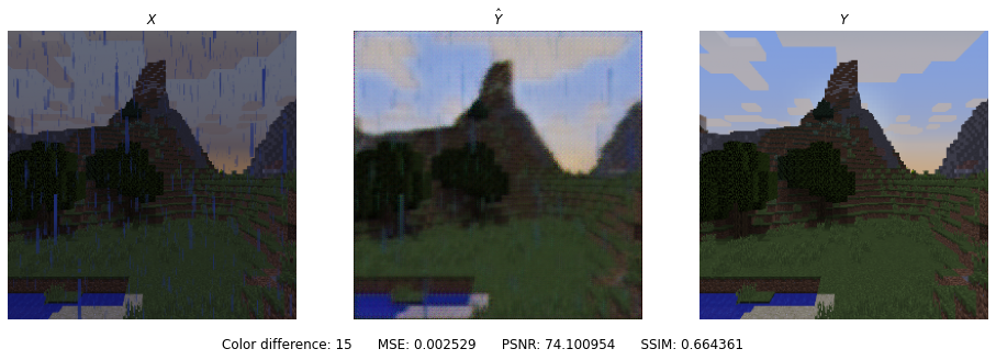
64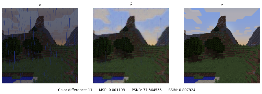
128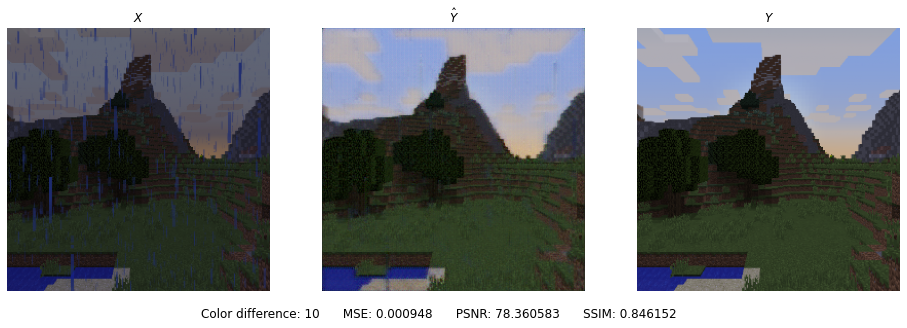

Summary of Results

With our experimentation, we have found the following combinations to produce the most optimal results:

• Loss Function: L1 only
• Batch Size: 5
• Learning Rate: 1e-3
• Filters in the last Conv layer: 128

With more data, we believe that our model would have been able to produce better results as 950 image pairs is small. Having more computational power would have allowed us to experiment with more data, epochs, filters, and layers. If we had more time, we would have liked to experiment with generating images of larger size (512x512) and running them on our model.

Best Run

For de-raining images:

For adding rain to images:

Resources Used

Godoy, D. (2019, February 07). Understanding binary cross-entropy / log loss: A visual explanation. Retrieved November 14, 2020, from https://towardsdatascience.com/understanding-binary-cross-entropy-log-loss-a-visual-explanation-a3ac6025181a

Image-to-Image Translation with Conditional Adversarial Networks. Phillip Isola, Jun-Yan Zhu, Tinghui Zhou, Alexei A. Efros. In CVPR 2017.

Unpaired Image-to-Image Translation using Cycle-Consistent Adversarial Networks. Jun-Yan Zhu, Taesung Park, Phillip Isola, Alexei A. Efros. In ICCV 2017. (* equal contributions)

What Are L1 and L2 Loss Functions? (n.d.). Retrieved November 14, 2020, from https://afteracademy.com/blog/what-are-l1-and-l2-loss-functions

What Are L1 and L2 Loss Functions? (n.d.). Retrieved November 14, 2020, from https://afteracademy.com/blog/what-are-l1-and-l2-loss-functions

Python

Peak Signal-to-Noise Ratio (PSNR) (n.d.). Retrieved December 15, 2020, from https://www.geeksforgeeks.org/python-peak-signal-to-noise-ratio-psnr/

A Quick Overview of Methods to Measure the Similarity Between Images (n.d.). Retrieved December 15, 2020, from https://medium.com/@datamonsters/a-quick-overview-of-methods-to-measure-the-similarity-between-images-f907166694ee